Synopsis

Bead sort, also called gravity sort, is a natural sorting algorithm, developed by Joshua J. Arulanandham, Cristian S. Calude and Michael J. Dinneen in 2002, and published in The Bulletin of the European Association for Theoretical Computer Science. Both digital and analog hardware implementations of bead sort can achieve a sorting time of O(n); however, the implementation of this algorithm tends to be significantly slower in software and can only be used to sort lists of positive integers. Also, it would seem that even in the best case, the algorithm requires O(n²) space.

Overview

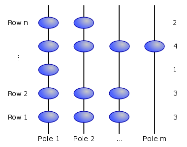
The bead sort operation can be compared to the manner in which beads slide on parallel poles, such as on an abacus. However, each pole may have a distinct number of beads. Initially, it may be helpful to imagine the beads suspended on vertical poles. In Step 1, such an arrangement is displayed using n=5 rows of beads on m=4 vertical poles. The numbers to the right of each row indicate the number that the row in question represents; rows 1 and 2 are representing the positive integer 3 (because they each contain three beads) while the top row represents the positive integer 2 (as it only contains two beads).

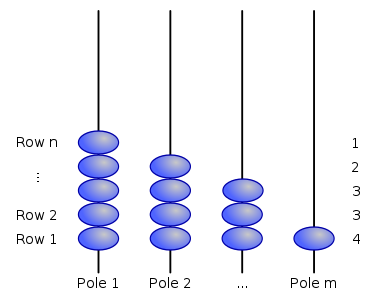
Step 1: Suspended beads on vertical poles.	Step 2: The beads have been allowed to fall.

If we then allow the beads to fall, the rows now represent the same integers in sorted order. Row 1 contains the largest number in the set, while row n contains the smallest. If the above-mentioned convention of rows containing a series of beads on poles 1..k and leaving poles k+1..m empty has been followed, it will continue to be the case here.

The action of allowing the beads to "fall" in our physical example has allowed the larger values from the higher rows to propagate to the lower rows. If the value represented by row a is smaller than the value contained in row a+1, some of the beads from row a+1 will fall into row a; this is certain to happen, as row a does not contain beads in those positions to stop the beads from row a+1 from falling.

he mechanism underlying bead sort is similar to that behind counting sort; the number of beads on each pole corresponds to the number of elements with value equal or greater than the index of that pole.

Complexity

Bead sort can be implemented with four general levels of complexity, among others:

• O(1): The beads are all moved simultaneously in the same time unit, as would be the case with the simple physical example above. This is an abstract complexity, and cannot be implemented in practice.
• O(sqrt{n}): In a realistic physical model that uses gravity, the time it takes to let the beads fall is proportional to the square root of the maximum height, which is proportional to n.
• O(n): The beads are moved one row at a time. This is the case used in the analog and digital hardware solutions.
• O(S), where S is the sum of the integers in the input set: Each bead is moved individually. This is the case when bead sort is implemented without a mechanism to assist in finding empty spaces below the beads, such as in software implementations.

Like the Pigeonhole sort, bead sort is unusual in that in worst case it can perform faster than O(n log n), the fastest performance possible for a comparison sort in worst case. This is possible because the key for a bead sort is always a positive integer and bead sort exploits its structure.

Implementations

• C

Notes

The Bead-Sort algorithm has drawn interest because of its promise of faster sorting times for positive integers, and as an excellent example of extracting an algorithm from a simple natural process (in this case, falling under the influence of gravity).

Speed and Complexity

There has been some confusion about the actual speed of the Bead-Sort algorithm. In their initial paper, Arulanandham, Calude, and Dinneen (ACD) suggested that depending on the user's perspective the sort might theoretically be considered O(1), O(n), O(S) or —that is, independent of the set size, varying linearly with it, or varying with the sum of the integers in the set. Since comparison sort methods are or (which is the best average case, as in quicksort, for instance), this is an exciting prospect, although it turns out to be unrealizable in software implementations. We consider the cases in turn:

O(1): This can only be justified by treating the falling of all the beads together as a single event independent of the number of beads, but it is difficult to see how it could be achieved in practice, even in a physical model, since the time necessary for an object to fall in a uniform gravitational field is proportional to the square root of the distance, and the beads would need to fall a maximum distance proportional to , making the physical model for the sorting stage, but for loading the inputs.

O(n): This can be realized in a hardware implementation that handles the columns in parallel. The ACD paper discusses two such hardware implementations (explained below), with the "beads" introduced one row at a time, each "bead" falling immediately to the lowest possible position in its column: behavior mimicked by the "hardware" mode in this Demonstration (although not actually realizable by software). If the beads are already in place, the parallel processing (as done by a hardware implementation) can still make the sort if at each step all beads above gaps fall simultaneously and immediately as far as the next lower bead. This is modeled visually by the "gap" setting.

Even if beads are only allowed to fall one position per time step, time may be saved if the setup and settling phases are not separated, if new rows are introduced one at a time at the top while the previously placed beads are still settling. The total time is no more than O(n+m), the sum of the number of rows and columns of the array, needing n time steps for the loading (while settling proceeds) followed by at most m time units for the remainder of the settling process after the last row enters the system—assuming comparable times for loading a new row and one settling step.

O(S): This is the best time that Bead-Sort can achieve without parallel treatment of columns: either introducing rows from the top, or with rows in place and beads scanned starting with the bottom row and continuing upward, we allow each bead to fall as far as it can. The time is proportional to S, the total number of beads, which is no more than n*m. (Straightforward software implementations are far more time intensive, however.)

Hardware Implementations

ACD proposed analog and digital hardware implementations using a graduated array of resistors or an array of triggered flip-flops, respectively, where rows of "beads" enter the top of the system and settle immediately to the lowest available level—not cascading down the columns one level at a time. This parallelization (treating all columns simultaneously) and short-circuiting the cascading process guarantees the O(n) sorting time. The analog implementation successively adds "beads" to resistor columns as voltage increments, which causes changes in the voltage levels across each resistor below, which then indicates the presence/absence of a bead at each position of the frame, given appropriate choices of voltage increment and threshold voltage, and the resistances to be used at each level. In the digital implementation, at each time step "beads" (0s or 1s) are loaded into a buffer register Bead[i] and then "dropped" into the main array of flip-flops, going directly to its final position in the array. This is achieved by a clever yet simple triggering condition for the individual cells: Cell[i,j] starts in the 0 state and will change to the 1 state if and only if And[Bead[i], Cell[i, j] == 0, Ceil[i, j-1] == 1].

Software Implementations

The direct software implementation of Bead-Sort is a two-dimensional cellular automaton (CA). ACD consider state changes of the entire CA as simultaneous, effectively requiring massive parallelization in order to again claim a sort time of O(n). However, in a nonparallelized algorithm, the whole n*m array must be scanned and updated for each CA update, giving a slow O(n2 m). This is what is actually happening behind the scenes in this Demonstration, although the image is only updated after each iteration of the whole array. In ill-behaved scenarios, beads may be temporarily blocked from falling by the presence of one or more beads beneath it that must fall first. (Run the Demonstration a few times, such cases occur rather frequently.)

Implementations that do not update the entire array at each step can have order O(m n). Treating only beads (i.e., filled cells, not empty cells) can reduce this to O(S), where is the sum of all the numbers to be sorted. But of course this is still slower than alternative sort schemes.

Besides the significantly slower software implementation, other drawbacks of the Bead-Sort algorithm that have been pointed out include a large memory requirement, O(m n)—or if an actual matrix transpose is performed, the larger of O(n2) and O(m2)—and the algorithm's (assumed) limitation to sets of positive integers. These difficulties have limited the practical value of Bead-Sort as a software algorithm.